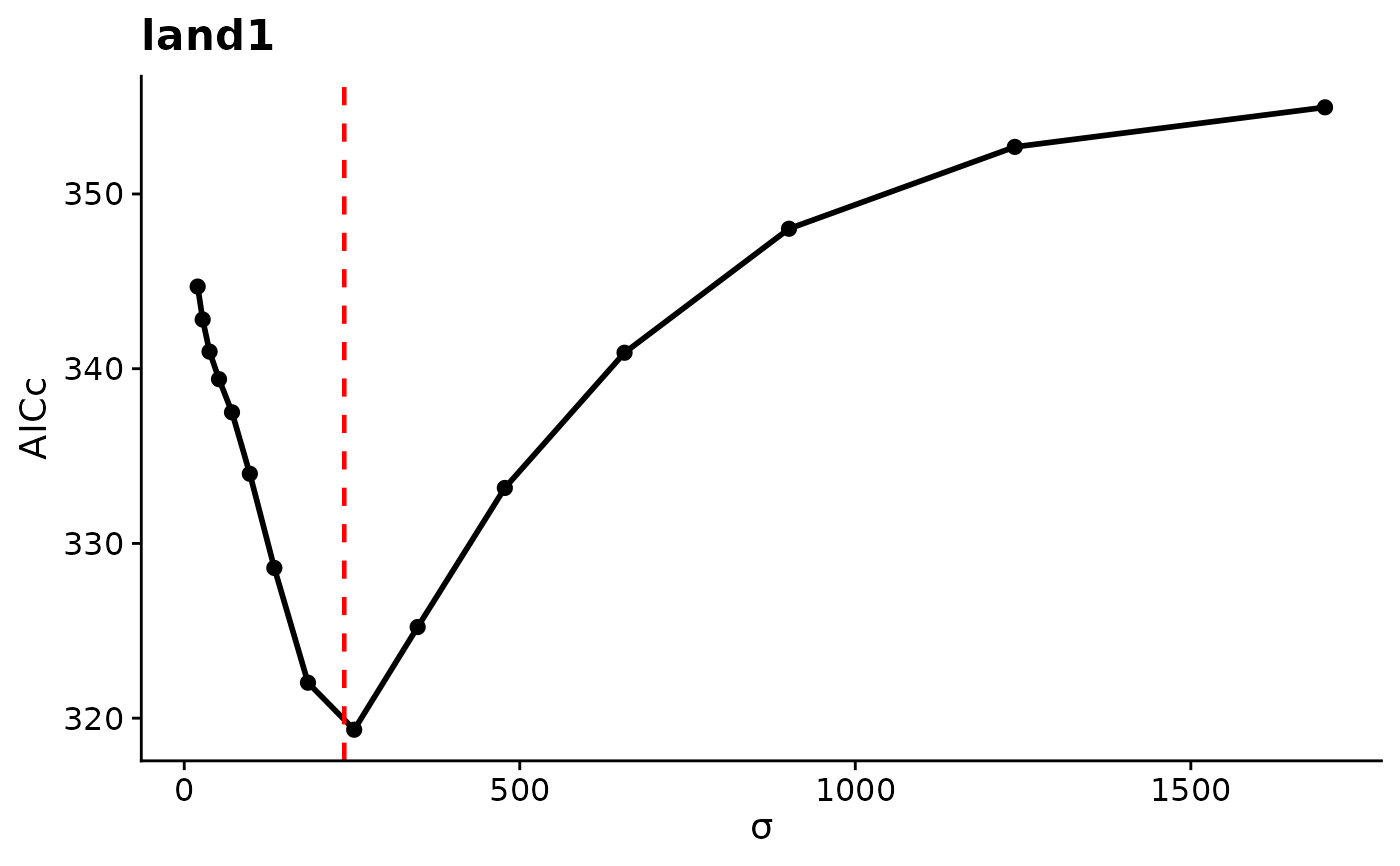
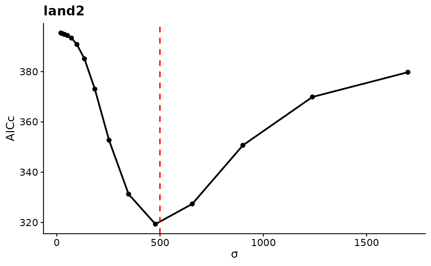
Draws one panel per covariate from a profile_sigma() result. Each panel
plots AICc or the log-likelihood (whichever metric was chosen in
profile_sigma()) against sigma, with points at the evaluated values and a
dashed red vertical line at the estimated sigma.
Usage
# S3 method for class 'sigma_profile'
plot(x, ...)
Arguments
- x
A
sigma_profileobject fromprofile_sigma().- ...
Not used.
Value
A named list of ggplot objects, one per covariate, returned
invisibly. Each plot is printed as a side effect. Modify a stored plot
and print it again to customize it.
Details
How to read the plot. The x-axis is sigma in map units, and the
y-axis is AICc (lower is better) or the log-likelihood (higher is better).
A clear trough in AICc, or peak in log-likelihood, at the dashed line means
the data identify the scale of effect well. A flat curve means many
scales fit about equally well. Points are joined with straight lines, so
a hard-radius covariate's stepped likelihood is not shown between grid
values. See profile_sigma() for how the values are computed.
Examples
## A stored profile from the Quick Start fit (two covariates, 15 values each)
prof <- readRDS(system.file("extdata", "cache-quickstart.rds",
package = "multiScaleR"))$prof
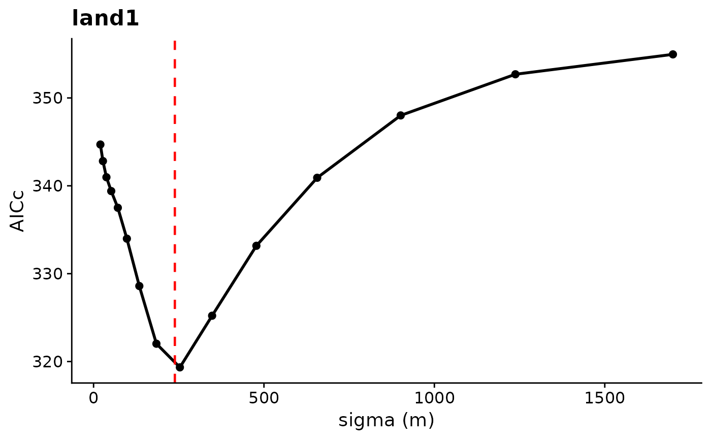
# One AICc panel each for land1 and land2. AICc is lowest near the
# estimated sigma (dashed line)
p <- plot(prof)
 # The stored ggplot objects can be modified and drawn again
p$land1 + ggplot2::labs(x = "sigma (m)")