
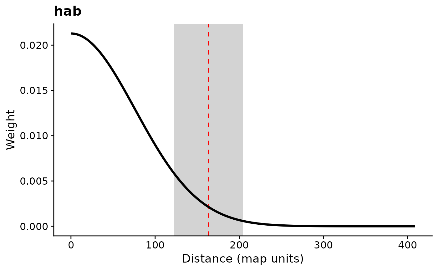
Plots the optimized kernel weight distribution for each spatial covariate in
a fitted multiScaleR object, with optional annotations showing the
effective scale of effect and its 95% confidence interval.
Arguments
- x
A fitted
multiScaleRobject returned bymultiScale_optim.- dimension
Character.
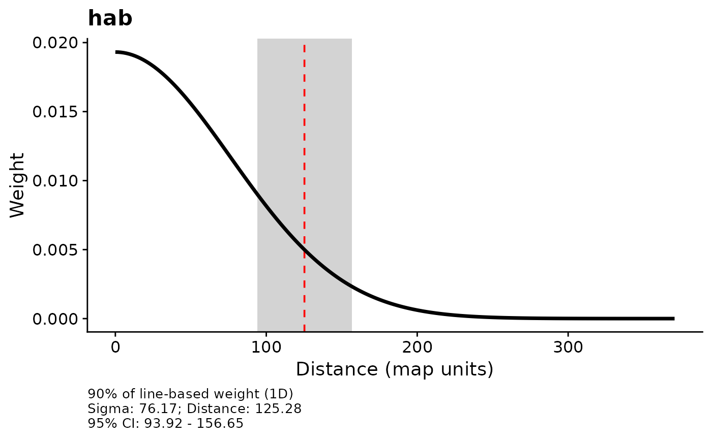
"2d"(default) marks the radius containing the requested proportion of ideal planar kernel weight."1d"restores the original distance along a line through the point.- ...
Optional named arguments to customize the plot:
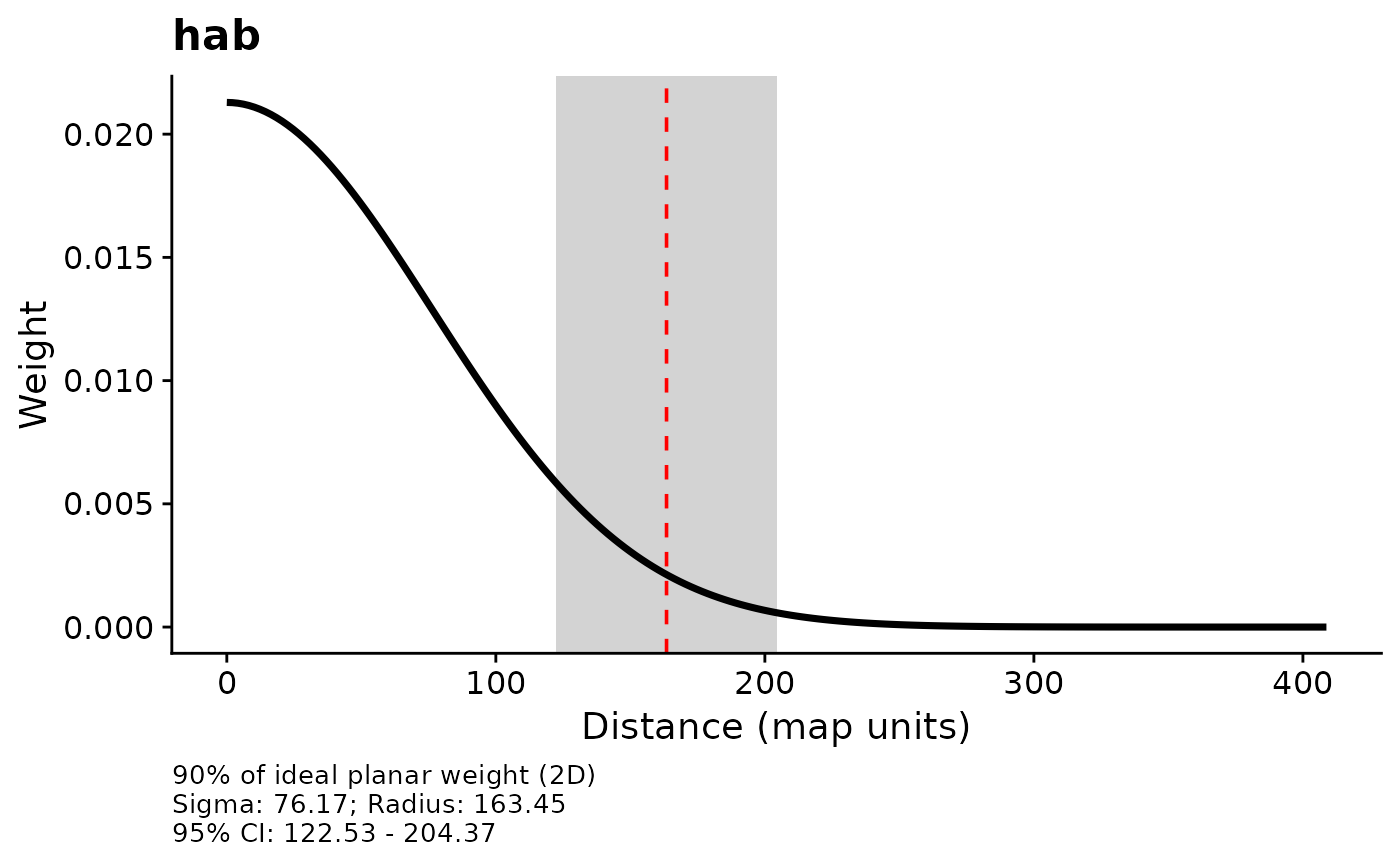
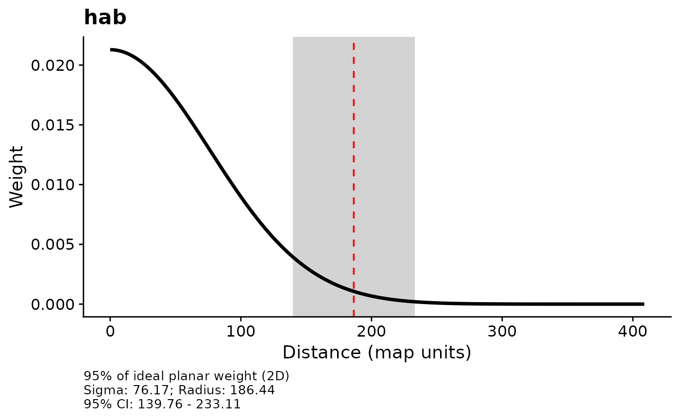
probNumeric between 0 and 1 (exclusive). Cumulative kernel weight enclosed by the marked distance under the selected
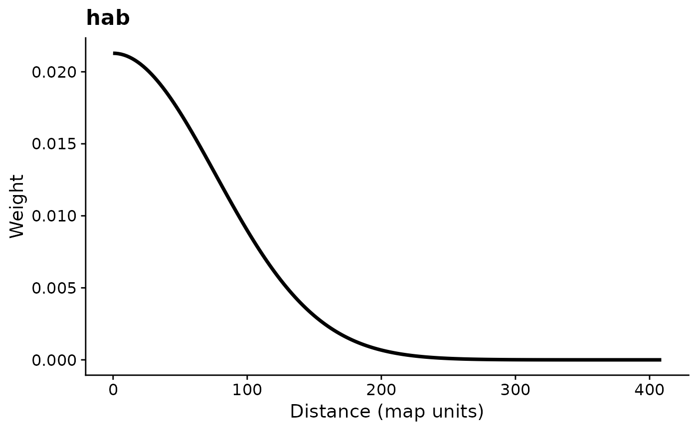
dimension. Default:0.9.scale_distLogical. If
TRUE(default), a vertical dashed line is drawn at the effective distance, and a shaded rectangle spans the 95% confidence interval.add_labelLogical. If
TRUE(default), a caption below the plot reports sigma, the dimensional definition, the effective distance, and 95% CI bounds (in map units).
Value
A list of ggplot2 objects (one per covariate with a finite
scale and effective distance), returned invisibly. Plots are printed as
a side effect.
Details
Development versions after 0.7.3 default to 2D reporting, as do
kernel_dist and plot_kernel. Set
dimension = "1d" to reproduce the original line-based distances.
This switch changes distance markers and converted confidence limits, not
the fitted sigma, regression coefficients, or likelihood.
The curve shows cell weight declining with distance, normalized over the
plotted sample distances. It is not a radial weight distribution. A planar
marker accounts for the increasing area of concentric rings, so the area
under the displayed curve to its left is not the stated proportion.
Distances refer to an ideal untruncated kernel. Actual retained weight can
differ with max_D, raster edges, missing cells, and cell geometry.
Hard-radius covariates, including every fitted fixed-kernel scale, show
a uniform buffer and mark its full radius,
regardless of prob or dimension. A shaded interval is drawn
only when finite limits are available.
Examples
# \donttest{
## Using package data
data('pts')
data('count_data')
hab <- terra::rast(system.file('extdata',
'hab.tif', package = 'multiScaleR'))
kernel_inputs <- kernel_prep(pts = pts,
raster_stack = hab,
max_D = 250,
kernel = 'gaussian')
#>
#> No sigma values provided...
#> Creating necessary elements to optimize sigma
#>
#> Extracting values from raster layers...
mod <- glm(y ~ hab,
family = poisson,
data = count_data)
## Optimize scale
opt <- multiScale_optim(fitted_mod = mod,
kernel_inputs = kernel_inputs)
#>
#>
#> Optimization complete
#>
#> WARNING!!!
#> The estimated scale of effect approaches or exceeds the current search extent.
#> Consider increasing max_D in `kernel_prep` to >=250.56 to ensure accurate estimation of scale.
#>
#>
plot(opt)
 plot(opt, dimension = "1d") # Original line-based distances
 plot(opt, prob = 0.95)
 plot(opt, scale_dist = FALSE)
 plot(opt, scale_dist = TRUE, add_label = FALSE)
 # }